BattleshipAI
This is an experiment in emergence. I have become increasingly interested in artificial neural networks and evolutionary algorithms, so I began a project to teach a computer how to play a game of Battleship.
Features
- Artificial neural network
- Battleship
- Training
The Game
Battleship is a game in which a player considers a grid containing some number of ships, and takes turns attacking individual cells with the goal of hitting all of the cells associated with each ship. We take the grid to contain n=64 cells arranged into an 8×8 square array. In the classic version of the game, the ships are the aircraft carrier (5 cells long), battleship (4), cruiser (3), submarine (3), and destroyer (2). We adopt this set of ships in all of our experiments. Thus, the total number of hits is h=17. Each ship can be arranged horizontally or vertically on the grid. Attacking any cell that does not contain part of a ship results in a miss.
A player's fitness is defined as the number of turns, on average, that are required to hit every ship cell. The goal of this project is to optimize the fitness function.
Random Control
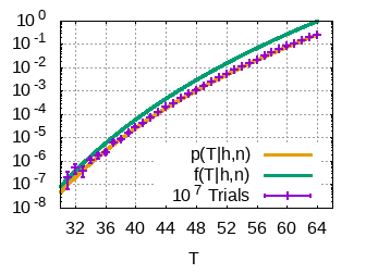
As a control case, we consider a player that attacks randomly. Here we derive the probability distribution for win success p(T|h,n), where T is a random variable representing the number of turns taken to hit h ship cells out of n total cells.
We can immediately deduce some properties of the distribution. The fact that any successful game must take at least as many turns as there are hits means that p(T<h|h,n)=0. At the start of a new game, each cell has probability h/n of containing a ship, so that the probability of getting a hit on the last remaining cell is p(T=n|h,n)=h/n. All games consist of at least T=h and at most T=n, and the probability distribution must satisfy
Now, let us calculate the probability of playing a perfect game. From the above considerations, the probability of getting a hit on the first turn is h/n. Now there are h-1 hits remaining and n-1 cells from which to choose, so the probability of getting a second hit is (h-1)/(n-1). Then, the combined probability of two hits in a row is simply the product of the individual probabilities. Continuing this pattern, we find that the probability of winning a game in T=h turns is
where the term in the denominator of the final expression is the binomial coefficient. Next, suppose that the player misses on the first turn, but then proceeds to win the game with h hits in a row. The probability of missing on the first turn is (n-h)/n, so that the probability of winning in T=h+1 turns is
Notice that the numerator of the first term cancels the denominator of the last term, which implies p(h+1|h,n)=p(h|h,n). Suppose, instead, that the player lands a hit on the first turn, misses the second, and then makes h-1 hits in a row to win. The probability is
By the commutativity of scalar multiplication, it is easy to see that the otherwise perfect game with a miss on the first turn has the same probability as the otherwise perfect game with a miss on the second turn. Naturally, this is true for a game with a single miss at any turn (except, of course, for the final turn, which is always a hit). Indeed, this trend is true for any number of misses, distributed in any order between hits.
The conclusion is that every possible individual game, consisting of a specific sequence of hits and misses, has the same probability. At first, it might seem surprising that a perfect game T=h has the same probability as a game taking T=n turns. Intuitively, the perfect game should be extremely unlikely compared to a game in which several misses occur. How do we reconcile the above analysis with our real-world expectations? The answer is multiplicity.
The key observation is that there are only a few ways to play a perfect game, but there are very many more ways to get misses. Consider the number of ways of distributing the misses into h bins, representing each possible game of length T. The probability of winning a game in T turns is then the probability of winning any particular game times the number of ways of playing a game of that length
With just a few well known binomial coefficient identities, it is easy to verify that this probability distribution satisfies all of the properties discussed at the beginning of this section. Thus, we claim that this distribution accurately models random gameplay. The cumulative distribution function can be represented in closed form as
We compare our distribution against the numerical experiments performed by DataGenetics. They simulate a Battleship game on n=100 cells arranged into a 10×10 grid. Their only analytical calculation is of the probability of a perfect game, and it agrees exactly with our result p(17|17,100). After playing 108 random games, they measure that roughly 50% of games complete in T=96, and 99% of games take more than T=78. Using our formula, we find f(96|17,100)=122508/261415≈46.8% and p(T>78|17,100)=1-f(78|17,100)=17541969854/17709002395≈99.1%. The results of our own experiments are shown in Fig. 1.